1.1. Principles of Data-Intensive Systems

CS 245 Principles of Data-Intensive Systems @ Stanford

2020 Winter

1.1.1. Intro

In many ways, data systems are the highest-level successful programming abstractions

How to Read a Paper: TLDR: don’t just go through end to end; focus on key ideas/sections

Two big ideas

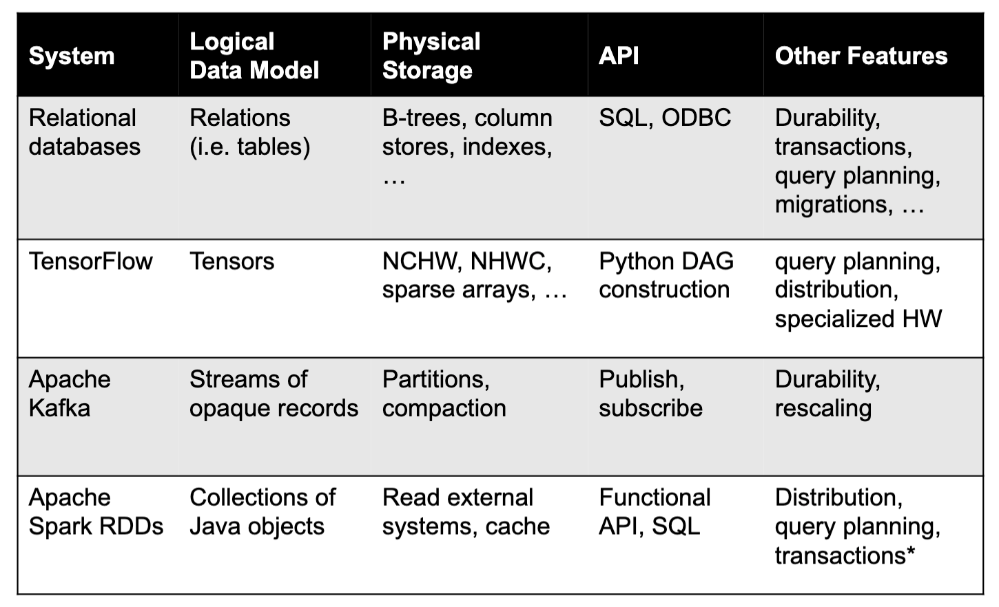
• Declarative interfaces (declarative APIs)
  • apps sepcify what they want, not how to do it
  • Example: “store a table with 2 integer columns”, but not how to encode it on disk;
  • SQL: Abstract “table” data model, many physical implementations; Specify queries in a restricted language that the database can optimize
  • TensorFlow: Operator graph gets mapped & optimized to different hardware devices
  • Functional programming (e.g. MapReduce): Says what to run but not how to do scheduling
  • Declaration instead of definition in code: make simple high-level abstraction and leave room for low-level optimization
• Transactions
  • Compress multiple actions into one atomic request
  • SQL db
  • Spark, MapReduce: Make the multi-part output of a job appear atomically when all partitions are done
  • Stream processing systems: Count each input record exactly once despite crashes, network failures, etc

Rest of the course

• Declarative interfaces
  • Data independence and data storage formats
  • Query languages and optimization
• Transactions, concurrency & recovery
  • Concurrency models
  • Failure recovery
  • Distributed storage and consistency

1.1.2. Database Archtecture

System R discussion

System R already has essential arch as a modern RDBMS

• SQL, cost-bases optimizer, compiling queries to asm
• many storate & access methods (b-trees), view-based access control
• lock manager, recovery via (write-ahead) logging / shadow pages (expensive for large files) (two for in-place updates)

Handling failures

• disk/storage media failure: main + backup disks
• system crash failure: shadow pages
• txn failure: log + lock

Tradeoff

• Fine-grained locking
  • lock records, fields, specific ops (R/W)
  • more concurrency, higher runtime overhead
• Coarse-grained locking
  • lock whole table for broader purposes (all ops)
  • more efficient to implement, less concurrency

Locking in System R

• Started with “predicate locks” based on expressions: too expensive
• Moved to hierarchical locks: record/page/table, with read/write types and intentions

Isolation in System R

• Level 1: Transaction may read uncommitted data; successive reads to a record may return different values
• Level 2: Transaction may only read committed data, but successive reads can differ
• Level 3: Successive reads return same value
• Most apps chose Level 3 (most strict) since others weren’t much faster

Authorization as alter to locking in concurrency

• Goal: give some users access to just parts of the db
• System R used view-based access control - define sql views for what the user can see and grant access
• Elegant implementation: add the user’s SQL query on top of the view’s SQL query

RDBMS arch

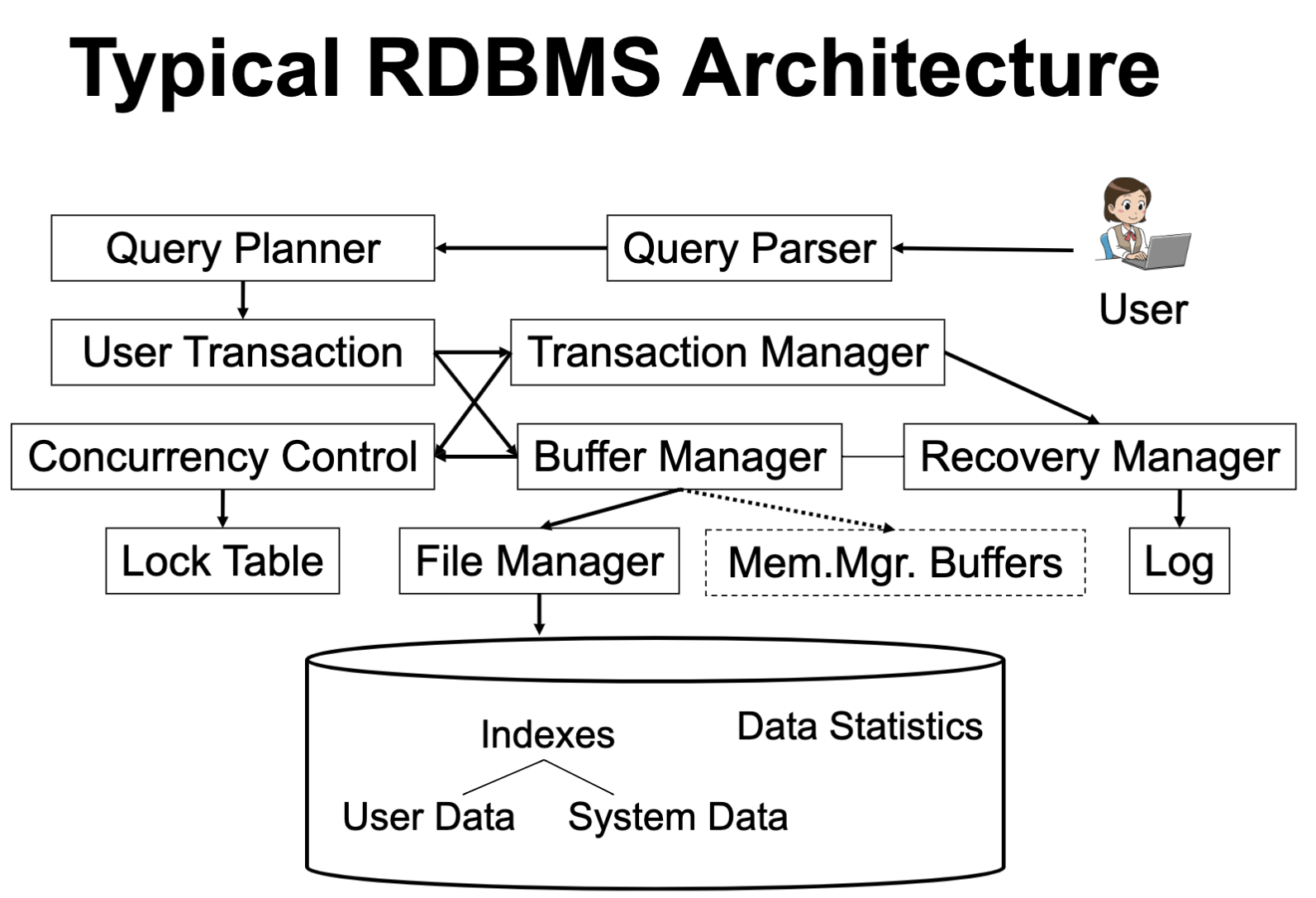
Boundaries

• Clear - modularity
  • SQL language, query plan representation, pages & buffers
• Vague - interact with others
  • Recovery + buffers + files + indexes
  • Txns + indexes
  • Data stat + query optimizer

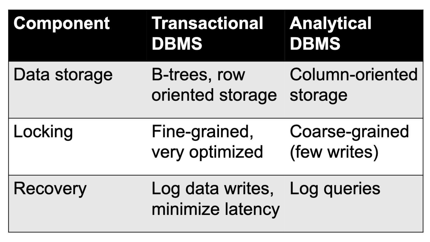
OLTP vs OLAP

• OLTP: focus on concurrent, small, low-latency transactions (e.g. MySQL, Postgres, Oracle, DB2) → real-time apps
• OLAP: focus on large, parallel but mostly read-only analytics (e.g. Teradata, Redshift, Vertica) → “data warehouses”

Alternative arch & tradeoffs

Potential ways to change DBMS arch

• Decouple query processing from storage management
  • 
  • Pros
    • Can scale compute independently of storage (e.g. in datacenter or public cloud)
    • Let different orgs develop different engines
    • Your data is “open” by default to new tech
  • Cons
    • Harder to guarantee isolation, reliability, etc
    • Harder to co-optimize compute and storage
    • Can’t optimize across many compute engines
    • Harder to manage if too many engines!
• Change the model
  • Key-value stores: data is just key-value pairs, don’t worry about record internals
  • Message queues: data is only accessed in a specific FIFO order; limited operations
  • ML frameworks: data is tensors, models, etc
  • Stream processing: apps run continuously and system can manage upgrades, scale-up, recovery, etc
  • Eventual consistency: handle it at app level
• Different hardware setting
  • Distributed databases: need to distribute your lock manager, storage manager, etc, or find system designs that eliminate them
  • Public cloud: “serverless” databases that can scale compute independently of storage (e.g. AWS Aurora, Google BigQuery)

1.1.3. Storage Formats & Indexing

Storage hardware

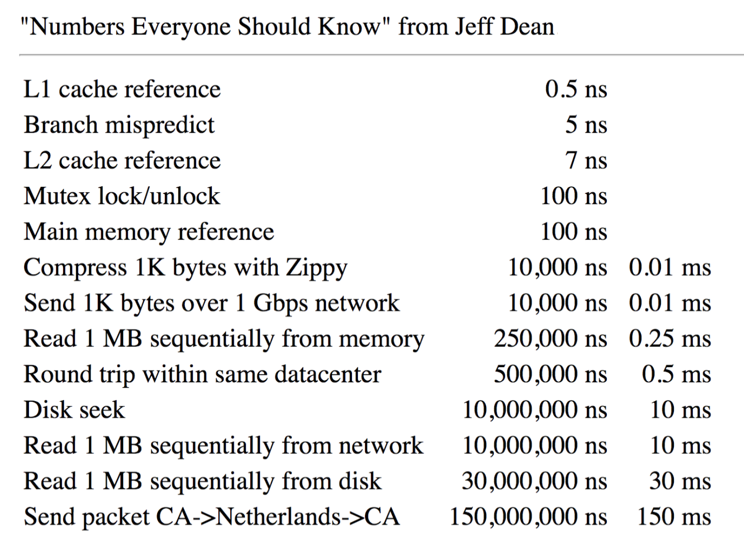
Max attainable throughput

• 100 GB/s for RAM
• 2 GB/s for NVMeSSD
• 130 MB/s for hard disk

Storage cost ($1000)

• 0.25 TB of RAM
• 9 TB of NVMe SSD
• 50 TB of magnetic disk

Hardware trends

• Capacity/$grows exponentially at a fast rate (e.g. double every 2 years)
• Throughput grows at a slower rate (e.g. 5% per year), but new interconnects help
• Latency does not improve much over time

Disk Access Time = Seek Time + Rotational Delay + Transfer Time + Other (details omitted)

The 5 Minute Rule for Trading MemoryAccesses for Disc Accesses (by Jim Gray & Franco Putzolu)

• Say a page is accessed every X seconds
• Assume a disk costs D dollars and can do I operations/sec; cost of keeping this page on disk is $C{d i s k}=C{i o p} / X=D /(I X)$
• Assume 1 MB of RAM costs M dollars and holds P pages; then the cost of keeping it in DRAM is $C_{m e m}=M / P$
• This tells us that the page is worth caching when $C{mem}< C{disk}$, i.e. $X<\frac{\text {PagesPerMBofDRAM}}{\text {AccessesPerSecondPerDisk}} \times \frac{\text {PricePerDiskDrive}}{\text {PricePerMBofDRAM}}$

Summary

• Storage devices offer various tradeoffs in terms of latency, throughput and cost
• In all cases, data layout and access pattern matter because random ≪ sequential access
• Most systems will combine multiple devices

Record encoding

Types of records

• Fixed/variable format/length
• Fixed format: A schema(not record) contains #/type/order/meaning of fields
• Variable format: Record itself contains format (self-describing)
  • Useful for “sparse” records, repeating fields, evolving formats, but may waste space
  • Format: record header + fields
  • Header: type (pointing to one of the schemas) + length + timestamps + concurrency stuff + etc.

Compression & encryption

Collection storage

Questions

• How do we place data items and records for efficient access?
  • Locality and searchability (quickly find relevant records, e.g. using sorting)
  • Locality - row/col store, hybrids (e.g. one field using col-store, the other two fields, potentially co-accessed, using row-store)
  • Searchability
    • Ordering
    • Partitions - place data into buckets based on a field (e.g. time, but not necessarily fine-grained order) - make it easy to add, remove & list files in any directory
    • Can We Have Searchability on Multiple Fields at Once?
      1. Multiple partition or sort keys (e.g. partition data by date, then sort by customer ID)
      2. Interleaved orderings such as Z-ordering
• How do we physically encode records in blocks and files?
  • Separating records
    • Fixed size records
    • Special marker
    • Given record lengths/offsets (within each rec. or in block header)
  • Spanned vs. unspanned
    • Unspanned - records must be within one block - simpler but waste space
    • Spanned - need indication of partial record - essential if rec. size > block size
  • Indirection - How does one refer to records? Physical vs. indirect.
    • Purely physical - record addr/id = {block id = {block/track/cylinder #}, offset in block}
    • Fully indirect - record id is arbitrary string - using map: id $\mapsto$ physical addr.
    • Tradeoff: flexibility (of moving records) vs. cost (of indirection)
  • Deletion and insertion

Summary

• There are 10,000,000 ways to organize my data on disk...
• Issues: flexibility, space utilization, complexity, performance
• Evaluation of a strategy
  • Space used for expected data
  • Expected time to
    • Fetch record given/next key
    • Insert/append/del/update records
    • Read all file
    • Reorganize file

Storage & compute co-design

C-Store (-> Vertica)

Compression

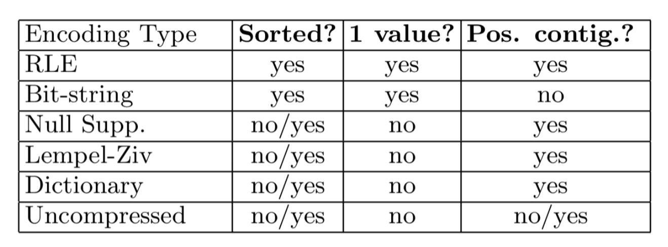
Indexes

Tradeoffs - size of indexes, cost to update indexes, query time

Types - conventional, b-trees, hash indexes, multi-key indexing

Sparse vs. dense

• Sparse better for insertion, dense needed for secondary indexes

With secondary indexes

• Lowest level is dense, other levels are sparse
• Pointers are record pointers (not block)
• Duplicate values - buckets

Conventional indexes

• Pros - simple, index is sequential (good for scan)
• Cons - expensive inserts, no balance

B-trees

• Motivation: give up sequential to get balanced

• B+ tree insertion/deletion

Hash indexes

• Hash vs tree indexes
  • O(1) disk access instead of O(logN)
  • Can't efficiently do range queries
• Resizing
  • Hash tables try to keep occupancy in a fixed range (50-80%) and slow down beyond that -> Too much chaining
  • How to resize?
    • In memory - just move everything, amortized cost is pretty low
    • On disk - moving everything is expensive
    • Extendible hashing - Tree-like design for hash tables that allows cheap resizing while requiring 2 IOs / access
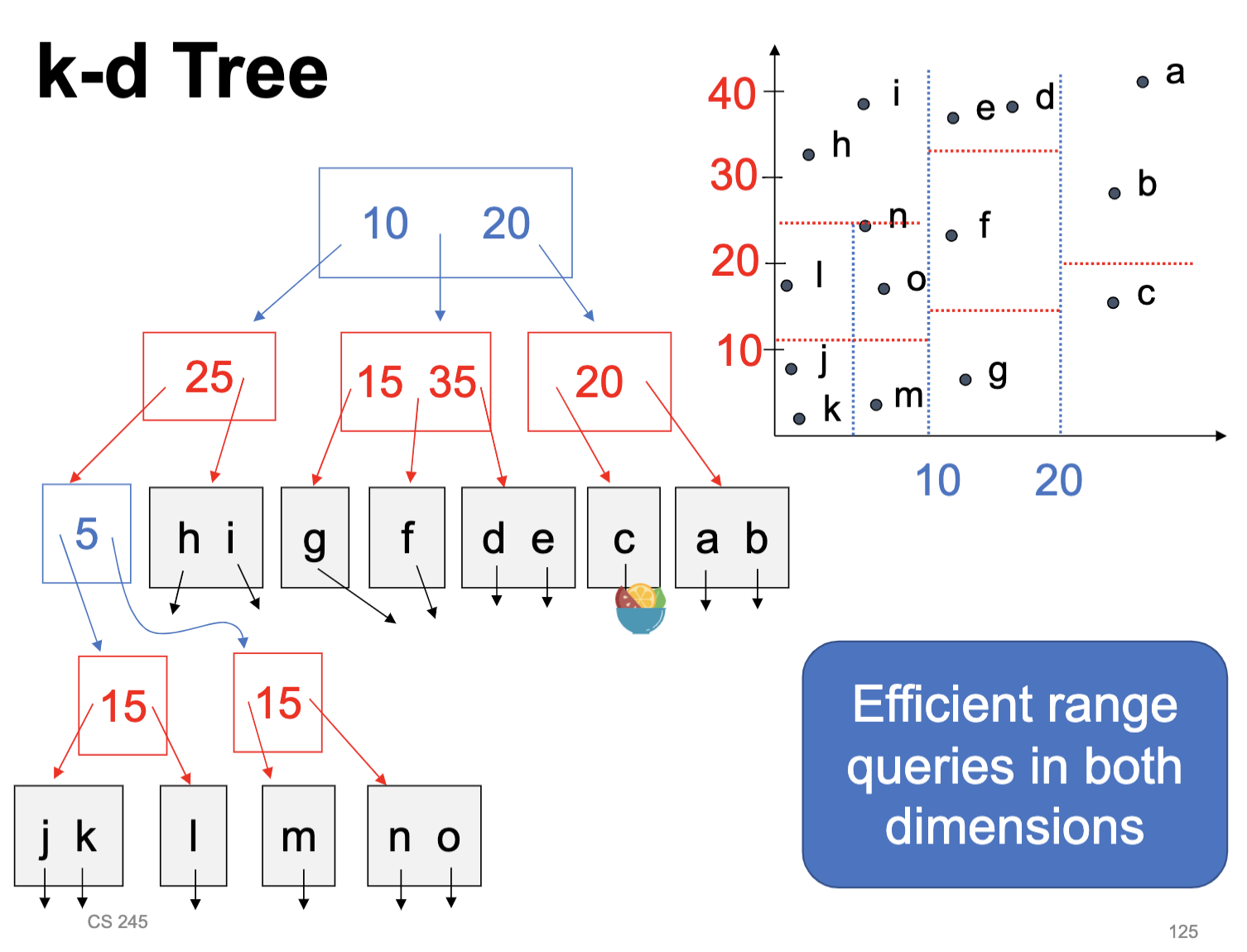
• Multi-key indexing
  • K-d tree - splits dimensions in any order to hold k-dimensional data
  • 

Storage system examples

• MySQL - transactional DBMS
  • Row-oriented storage with 16 KB pages
  • Variable length records with headers, overflow
  • Index types - B-tree, hash (in-memory only), R-tree (spatial data), inverted lists for full text search
  • Can compress pages with Lempel-Ziv
• Apache Parquet + Hive - analytical data lack
  • Col-store as set of ~1 GB files (each file has s slice of all columns)
  • Various compression and encoding schemes at the level of pages in a file
    • Special scheme for nested fields (Dremel)
  • Header with statistics at the start of each file
    • Min/max of columns, nulls, Bloom filter
  • Files partitioned into directories by one key

1.1.4. Query Execution & Optimization

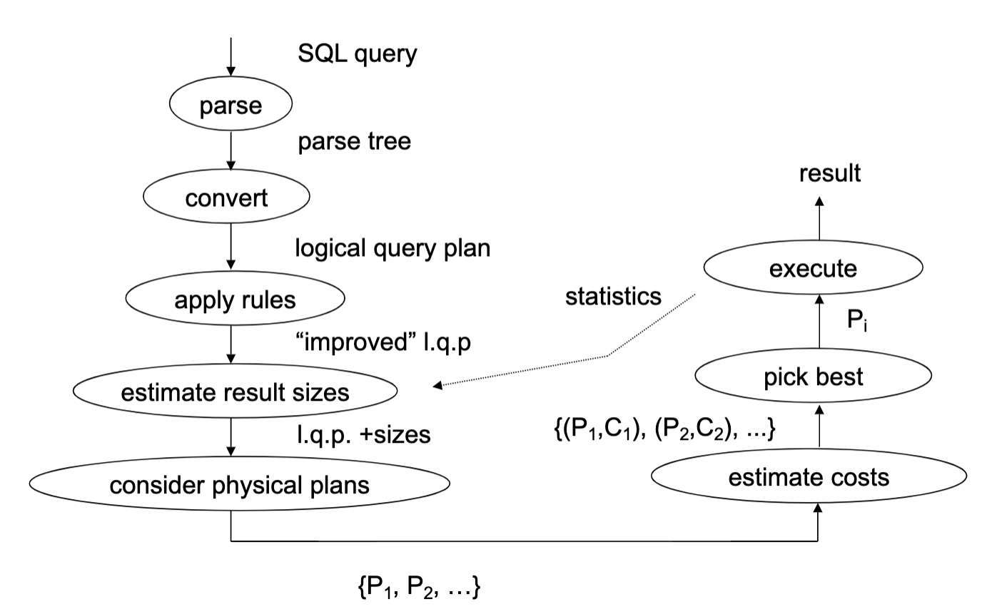
Overview

Query execution overview

1. Query representation (e.g. SQL)
2. Logical query plan (e.g. relational algebra)
3. Optimized logical plan
4. Physical plan (code/operators to run)
   • Many execution methods - per-record execution, vectorization, compilation

Plan optimization methods

• Rule-based - systematically replace some expressions with other expressions
  • X OR TRUE -> TRUE, M*A + M*B -> M*(A+B)
• Cost-based - propose several execution plans and pick best based on a cost model
• Adaptive - update execution plan at runtime

Execution methods

• Interpretation - walk through query plan operators for each record
• Vectorization - walk through in batches
• Compilation - generate code (like in System R)

Typical RDBMS execution

Relational operators

Relational algebra

• Codd's original - tables are sets of tuples; unordered and tuples cannot repeat
• SQL - tables are bags (multi-sets) of tuples; unordered but each tuple may repeat

Operators

• Intersection, union, difference, Cartesian Product
• Selection, projection, natural join, aggregation
• Properties

SQL query example

• Find the movies with stars born in 1960 SELECT title FROM Stars In WHERE starName IN (SELECT name FROM MovieStar WHERE birthdate LIKE ‘%1960’);
• Parse tree
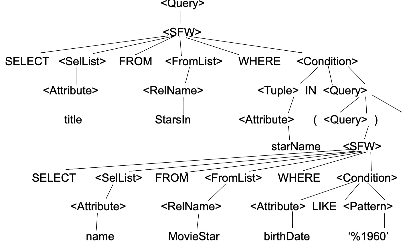
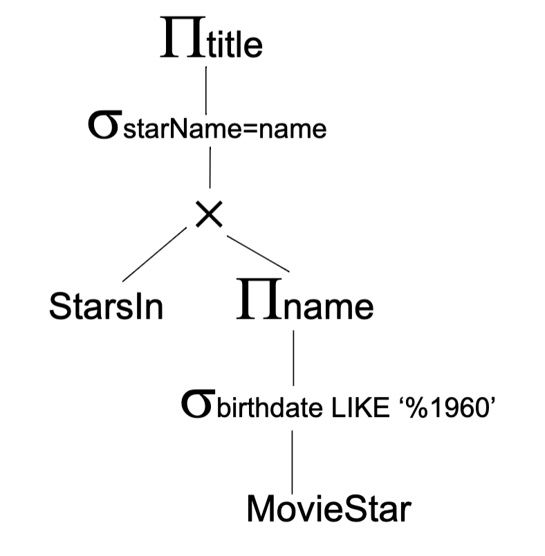
• Logical query plan
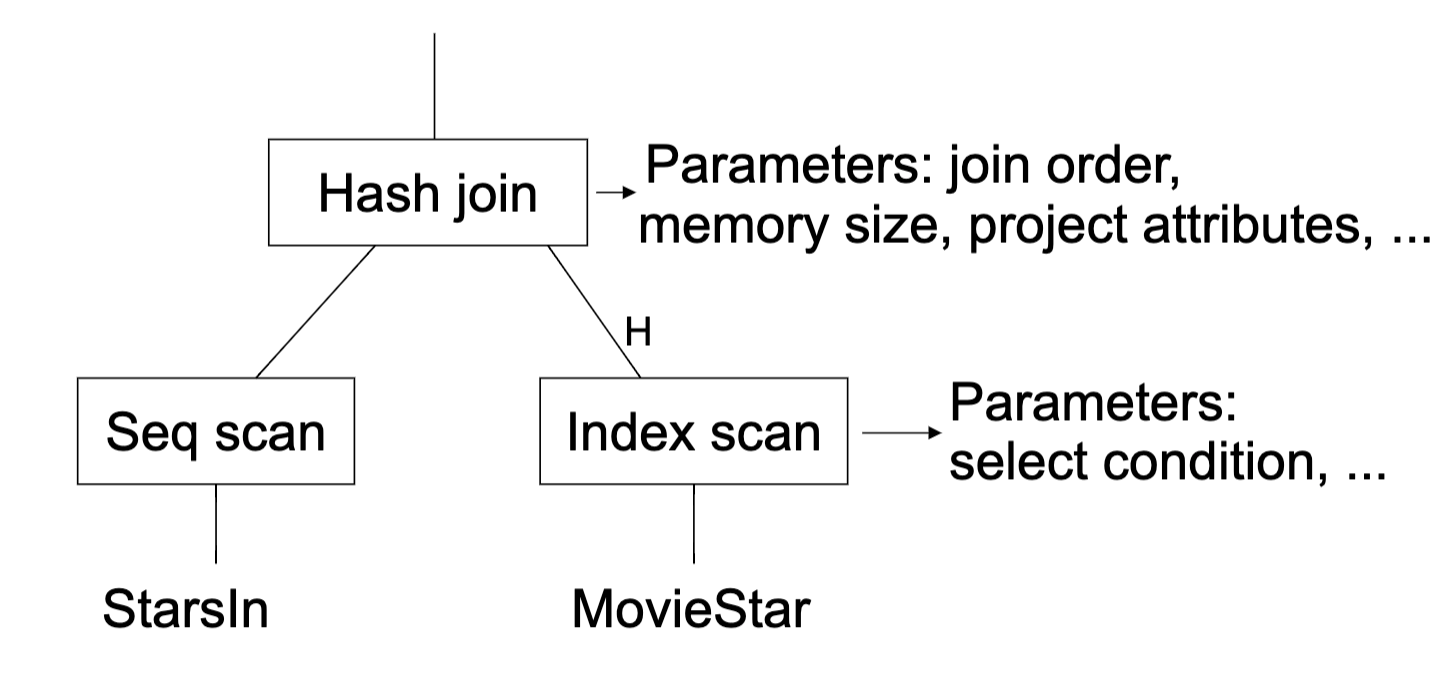
• Physical plan (Index scan and sequence scan can swap)

Execution methods

• Interpretation
  • Recursively calls Operator.next() and Expression.compute()
• Vectorization
  • Interpreting query plans one record at a time is simple but also slow
    • Lots of virtual function calls and branches for each record
  • Keep recursive interpretation, but make Operators and Expressions run on batches
  • Implementation
    • Tuple batches fit in L1 or L2 cache
    • Operators use SIMD instructions to update both values and null fields without branching
  • Pros - Faster when processing many records, relatively simple to implement
  • Cons - Lots of nulls in batches if query is selective, data travels between CPU & cache a lot
• Compilation
  • Turn the query into executable code
  • Pros - potentially fastest, leverage modern compilers
  • Cons - complex to implement, compilation takes time, generated code may not match hand-written

Modern choice

• OLTP (MySQL) - mostly record-at-a-time interpretation
• OLAP (Vertica, Spark SQL) - vectorization, sometimes compilation
• ML libs (TensorFlow) - mostly vectorization (records are vectors), sometimes compilation

Optimize target

Target

• Operator graph - what operators do we run, and in what order?
• Operator implementation - for operators with several implementations (e.g. join), which one to use?
• Access paths - how to read each table? Index scan, table scan, C-store projections, etc.

Challenge

• Exponentially large set of possible query plans (...similar to TASO)
• We need techniques to prune the search space and complexity involved

Rule-based optimization

Rule (...pattern or template)

• Def - Procedure to replace part of the query plan based on a pattern seen in the plan

• Implementation

  • Each rule is typically a function that walks through query plan to search for its pattern.
  • Rules are often grouped into phases (e.g. simplify boolean expressions, pushdown selects, choose join algorithms)
  • Each phase run rules till they no longer apply
  • Combined simple rules can optimize complex query plans (if designed well)

• Example - Spark SQL's Catalyst Optimizer

  • Written in Scala to use its pattern matching

  • > 1000 types of expressions, hundreds of rules

Common rule-based optimizations

• Simplifying expressions in select, project, etc
  • Boolean algebra, numeric expressions, string expressions, etc.
  • Many redundancies because queries are optimized for readability or generated by code
• Simplifying relations operators graphs
  • Select, project, join, etc. - These relational optimizations have the most impact
• Simplifying access patterns and operator implementations in simple cases - Also very high impact
  • Index column predicate -> use index
  • Small table -> use hash join against it
  • Aggregation on field with few values -> use in-memory hash table
• Rules also often used to do type checking and analysis (easy to write recursively)

Common relational rules

• Push selects as far down the plan as possible - reduce # of records early to minimize work in later ops; enable index access paths
• Push projects as far down as possible - don't process fields that you'll just throw away
• Be careful - project rules can backfire

Bottom line

• Many possible transformations aren't always good for performance
• Need more info to make good decisions
  • Data stats - properties about our input or intermediate data to be used in planning
  • Cost models - how much time will an operator take given certain input data stats?

Data statistics

Data stats

• Def - info about tuples in a relation that can be used to estimate size and cost
• Example - # of tuples, avg size of tuples, # distinct values for each attribute, % of null values for each attribute
• Typically maintained by the storage engines as tuples are added/removed in a relation
  • File formats like Parquet (col-stored) can also have them
• Challenge - how to keeps stats for intermediate tables during a query plan?
• Stat estimation methods based on assumptions (should balance speed, accuracy and consistency)
  • Omitted. Please refer to examples in slides.

Cost models

How do we measure a query plan's cost?

• # disk IOs (focus), # of compute cycles
• Combined time metric, memory usage, bytes sent on network
• Example - index vs table scan

Join operators

• Join orders and algorithms are often the choices that affect performance the most
• Common join algorithms
  • Iterator (nested loops) join - cost = [B(R1) + T(R1) B(R2)] reads + [B(R1⨝R2)] writes
  • Merge join - cost = [B(R1) + B(R2)] reads + [B(R1⨝R2)] writes + (if not sorted, 4B(Ri) I/Os)
  • Join with index - read cost = B(R1) + T(R1) (L~index~+ L~data~)
  • Hash join - read cost = B(R1) + B(R2)
    • Hash join in memory/disk
    • Trick: hash (key, pointer to records) and sort pointers to fetch sequentially
  • If joins very selective, may prefer methods that join pointers or do index lookups

In general, the following are used

• Index join if an index exists
• Merge join if at least one table is sorted
• Hash join if both tables unsorted

Cost-based plan selection

Process - generate plans -> prune -> estimate cost -> pick min cost

How to generate plans

• Can limit sear space - many dbs only consider left-deep joins
• Can prioritize searching through the most impactful decisions first - e.g. join order

How to prune

• Throw current plan away if it's worse than best so far
• Use greedy to find an "OK" initial plan that will allow lots of pruning
• Memoization - remember cost estimates and stats for repeated subplans
• Dynamic programming - can pick an order to subproblems to make it easy to reuse results

Resource cost

• It's possible for cost-based optimization itself to take longer than running the query.
• Luckily, a few big decisions drive most off the query execution time (e.g. join order)

Spark SQL

History

Resilient distributed datasets (RDDs)

• Immutable collections of objects that can be stored in memory/disk across a cluster
• Bulit with parallel transformations (map, filter, etc.)
• Automatically rebuilt on failure

Challenges with Spark's original functional API

• Looks high-level, but hides many semantics of computation from engine
  • Functions passed in are arbitrary blocks of code
  • Data stored is arbitrary java/python objects. Java objects often many times larger than data.
• Users can mix APIs in suboptimal ways

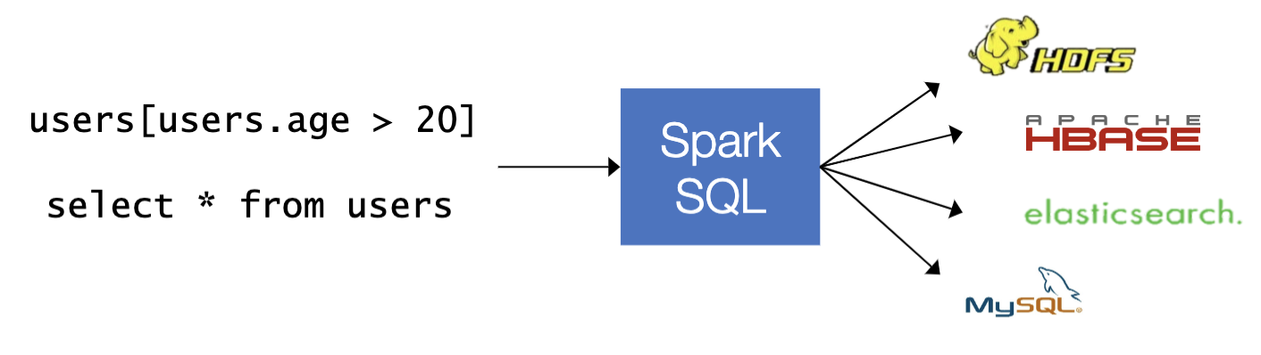
Spark SQL & DataFrames - efficient lib for working with structured data

• 2 interfaces: SQL for data analysts and external apps, DataFrames for complex programs

• Optimized computation and storage underneath

• 

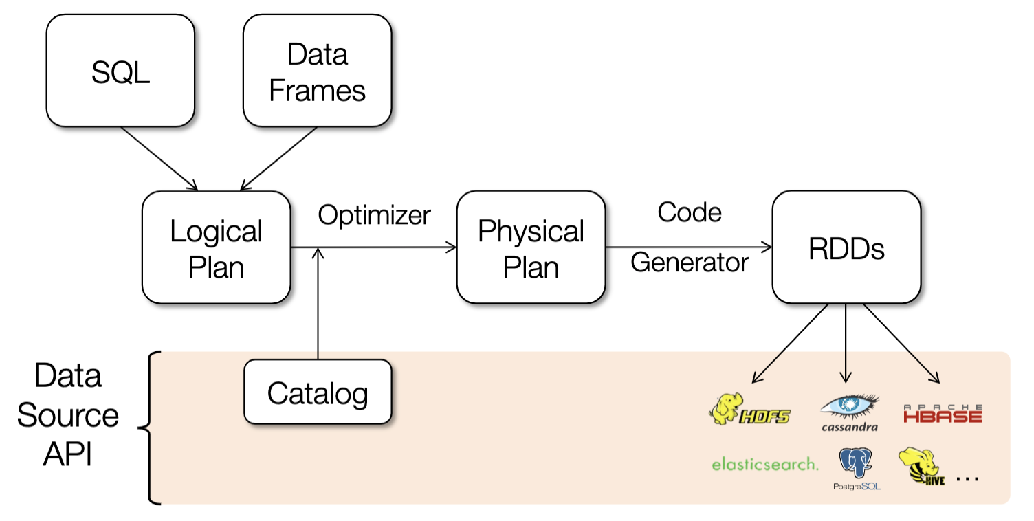
• DataFrames hold rows with a known schema and offer relational operations through a DSL

  • Based on data frame concept in R, python, Spark is the first to make this declarative
  • Integrated with the rest of Spark - ML lib, easily convert RDDs

• What DataFrames Enable

  • Compact binary representation - columnar, compressed cache; rows for processing
  • Optimization across operators (join reordering, predicate pushdown, etc)
  • Runtime code generation

• Uniform ways to access structured data

  • Apps can migrate across Hive, Cassandra, Json, Parquet

  • Rich semantics allows query pushdown into data sources.

  • 

Extensions to Spark SQL

• Tens of data sources using the pushdown API
• Interval queries on genomic data, Geospatial package (Magellan)
• Approximate queries & other research

1.1.5. Transactions & Recovery

Defining correctness, transaction model, hardware failures, recovery with logs, undo/redo logging

Def, undo logging, redo logging, checkpoints

Problems with ideas so far

• Undo logging: need to wait for lots of I/O to commit; can’t easily have backup copies of DB
• Redo logging: need to keep all modified blocks in memory until commit

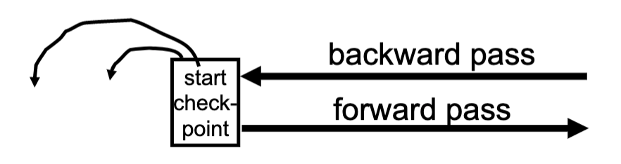
-> Undo/redo logging

1. Backward pass (end of log → latest valid checkpoint start)
   • construct set S of committed transactions
   • undo actions of transactions not in S
2. Undo pending transactions
   • follow undo chains for transactions in(checkpoint’s active list) -S
3. Forward pass (latest checkpoint start → end of log)
   • redo actions of all transactions in S
4. 

Media failures = Loss of nonvolatile storage -> make copies

When can logs be discarded?

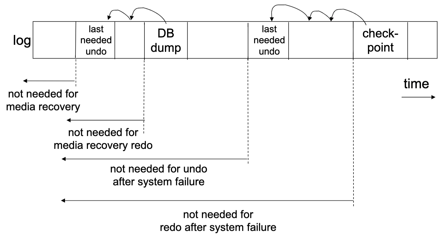
Summary = logging + redundancy

For details about this section, please refer to slides or any common database courses.

1.1.6. Concurrency

Isolation levels

• Strong isolation - easier to reason about (can't see others' change)
• Weak isolation - see others' changes, but more concurrency
• Virtually no commercial DBs do serializability by default, and some can’t do it at all

Serializability

Concepts

• Transaction: sequence of r~i~(x), w~i~(x) actions
• Schedule:a chronological order in which all the transactions’ actions are executed
• Conflicting actions: pairs of actions that would change the result of a read or write if swapped
• Schedules S1, S2 are conflict equivalent if S1can be transformed into S2by a series of swaps of non-conflicting actions(i.e., can reorder non-conflicting operations in S1 to obtain S2)
• A schedule is conflict serializable if it is conflict equivalent to some serial schedul
• Precedence graphs
  • If S1, S2 conflict equivalent, then P(S1) = P(S2). But the reverse is not true
  • P(S1) acyclic <=> S1 conflict serializable

2PL & OCC

2PL

• Def, correctness proof
• Optimzing performance
  • Shared locks
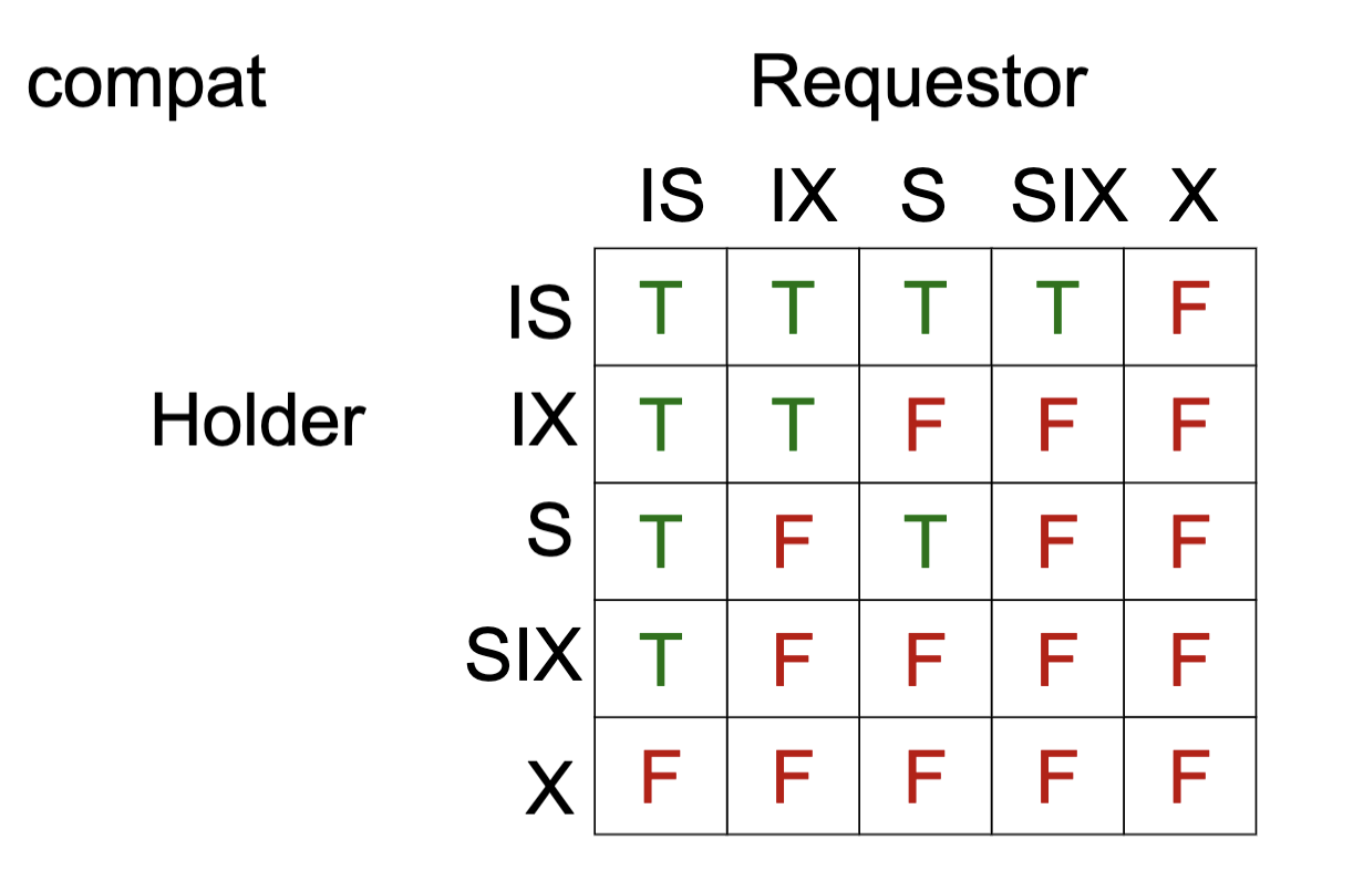
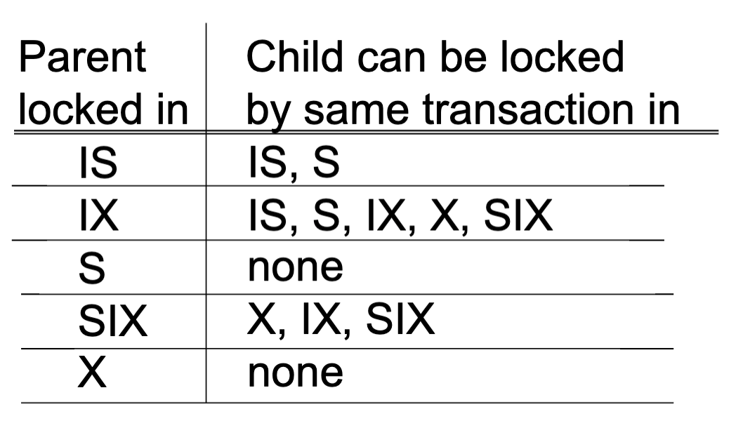
  • Multiple granularity
    • Tree representation - fields, tuples, tables, relations...
  • Lock variants
  • Inserts, deletes and phantoms
  • Other types of C.C. mechanisms

Validation performs better than locking when

• Conflicts are rare
• System resources are plentiful
• Have tight latency constraints

For details about this section, please refer to slides or any common database courses.

Concurrency control & recovery

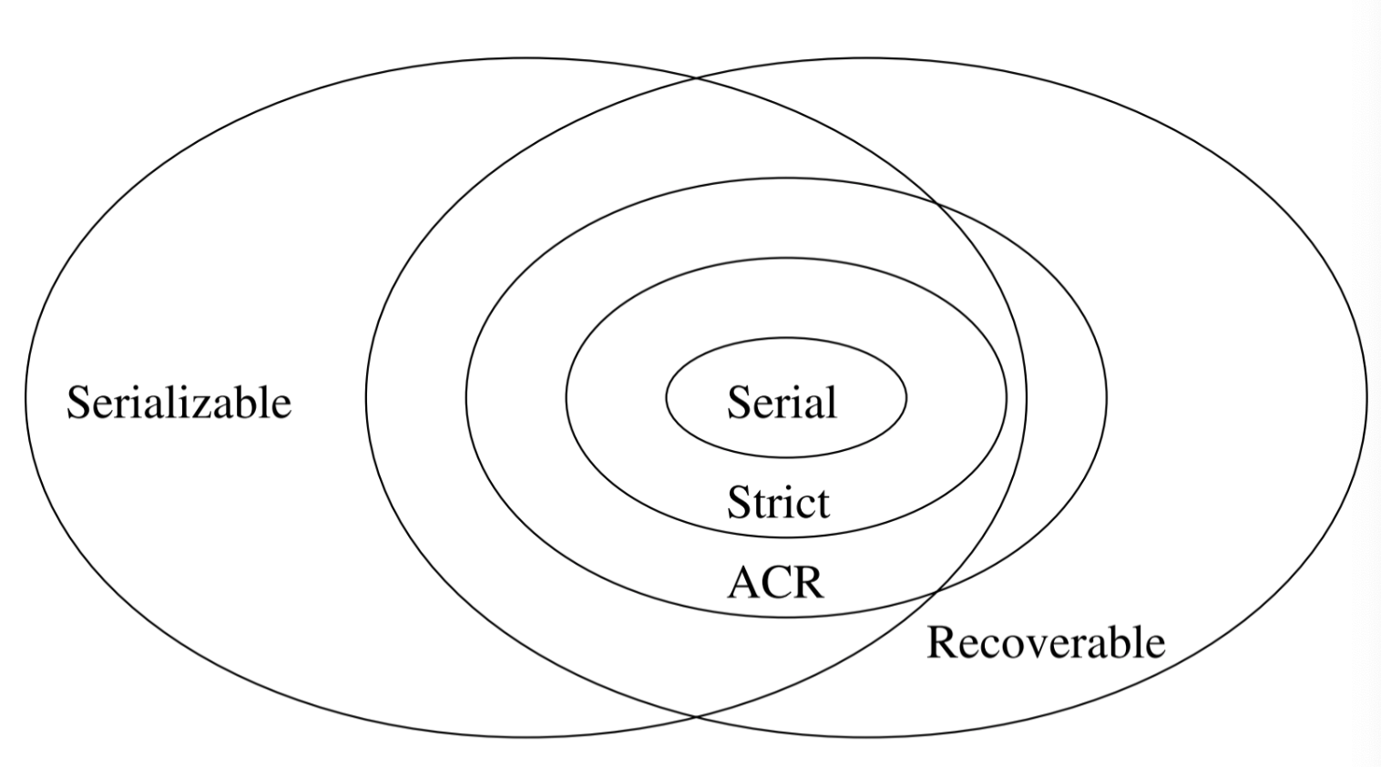
Recoverable schedule

• S is recoverable if each transaction commits only after all transactions from which it read have committed
• S avoids cascading rollback if each transaction may read only those values written by committed transactions
• S is strict if each transaction may read and write only items previously written by committed transactions (≡ strict 2PL)
• With OCC, no actions is needed. Each transaction’s validation point is its commit point, and only write after.
• Serial ⊂ strict ⊂ avoids cascading rollback ⊂ recoverable
• Example
  • Recoverable: w1(A) w1(B) w2(A) r2(B) c1c2
  • Avoids Cascading Rollback: w1(A) w1(B) w2(A) c1 r2(B) c2
  • Strict: w1(A) w1(B) c1w2(A) r2(B) c2
• Every strict schedule is serializable.
• 

Beyond serializability

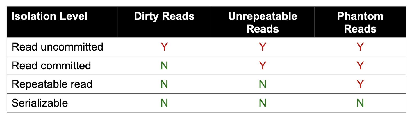
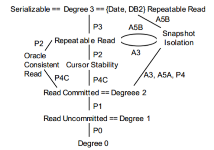
Weaker isolation levels

• Dirty reads
  • Let transactions read values written by other uncommitted transactions
  • Equivalent to having long-duration write locks, but no read locks
• Read committed
  • Can only read values from committed transactions, but they may change
  • Equivalent to having long-duration write locks (X) and short-duration read locks (S)
• Repeatable reads
  • Can only read values from committed transactions, and each value will be the same if read again
  • Equivalent to having long-duration read & write locks (X/S) but not table locks for insert
• Snapshot isolation
  • Each transaction sees a consistent snapshot of the whole DB (as if we saved all committed values when it began)
  • Often implemented with MVCC

Facts

• Oracle calls their snapshot isolation level “serializable”, and doesn’t provide serializable
• Many other systems provide snapshot isolation as an option
  • MySQL, PostgreSQL, MongoDB, SQLServer

For details about this section, please refer to slides or any common database courses.

1.1.7. Distributed Systems

Replication

General problem: how to tolerate server/network failures

The eight fallacies of distributed computing (by Peter Deutsch)

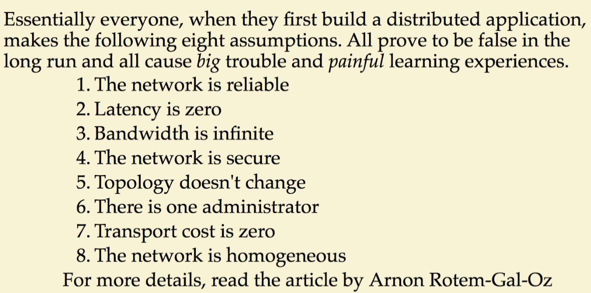
Replication

• Primary-backup
  • 1 primary + n backup
  • send requests to primary, which then forwards operations or logs to backups
  • Sync/async backup coordination
• Quorum replication
  • Read and write to intersecting sets of servers; no one “primary”
  • Common: majority quorum - More exotic ones exist, like grid quorums
  • Surprise: primary-backup is a quorum too!
  • Eventual consistency - If writes stop, eventually all replicas will contain the same data - async broadcast all write to all replicas

Solutions to failures - consensus

• {Paxos, Raft} + {modern implementations: Zookeeper, etcd, Consul}
• Idea - keep a reliable, distributed shared record of who is primary
• Distributed agreement on one value/log of events

Partitioning

Split database into chunks called partitions

• Typically partition by row
• Can also partition by column (rare)

Partition strategies

• Hash key to servers - random assignment
• Partition keys by range - keys stored contiguously
• What if servers fail (or we add servers)? - Rebalance partitions using consensus.

Distributed transactions

• Replication
  • Must make sure replicas stay up to date
  • Need to reliably replicate the commit log (using consensus or primary-backup)
• Partitioning
  • Must make sure all partitions commit/abort
  • Need cross-partition concurrency control

Atomic commitment & 2PC

Atomic commitment (in a distributed transaction) - Either all participants commit a transaction, or none do

2PC + OCC

• Participants perform validation upon receipt of prepare message
• Validation essentially blocks between prepare and commit message

2PC + 2PL

• Traditionally: run 2PC at commit time
  • i.e., perform locking as usual, then run 2PC to have all participants agree that the transaction will commit
• Under strict 2PL, run 2PC before unlocking the write locks

2PC + logging

• Log records must be flushed to disk on each participant before it replies to prepare
• The participant should log how it wants to respond + data needed if it wants to commit

Optimizations

• Participants can send prepared messages to each other
  • Can commit without the client
  • Requires O(P^2^) messages
• Piggyback transaction’s last command on prepare message
• 2PL - piggyback lock “unlock” commands on commit/abort message

Possible failures - unavailable coordinators/participants, or both

Every atomic commitment protocol is blocking(i.e., may stall) in the presence of

• Asynchronous network behavior (e.g., unbounded delays) -> Cannot distinguish between delay and failure
• Failing nodes -> If nodes never failed, could just wait

CAP

Async network model

• Message can be arbitrary delayed
• Can't distinguish between delayed messages and failed nodes in a finite amount of time

CAP Theorem

• In an async network, a distributed database can either (not both)
  • guarantee a response from any replica in a finite amount of time (“availability”) OR
  • guarantee arbitrary “consistency” criteria/constraints about data
• Choose either
  • Consistency and “Partition Tolerance”
  • Availability and “Partition Tolerance”
• “CAP” is a reminder - No free lunch for distributed systems

Why CAP is important

• Pithy reminder: “consistency” (serializability, various integrity constraints) is expensive!
  • Costs us the ability to provide “always on” operation (availability)
  • Requires expensive coordination (synchronous communication) even when we don’t have failures

Avoiding coordination

Why need avoid coordination

• How fast can we send messages? - Planet Earth: 144ms RTT
• Message delays often much worse than speed of light (due to routing)
• Key finding - most applications have a few points where they need coordination, but many operations do not.
• Serializability has a provable cost to latency, availability, scalability (if there are conflicts)
• We can avoid this penalty if we are willing to look at our application and our application does not require coordination
  • Major topic of ongoing research

BASE idea = “Basically Available, Soft State, Eventual Consistency”

• Partition data so that most transactions are local to one partition (reduce # of cross-partition txns)
• Tolerate out-of-date data (eventual consistency)
  • Caches, weaker isolation levels (causal consistency), helpful ideas (idempotence, commutativity)
• BASE Example
  • Constraint:each user’s amt_sold and amt_bought is sum of their transactions
  • ACID Approach - to add a transaction, use 2PC to update transactions table + records for buyer, seller
  • One BASE approach - to add a transaction, write to transactions table + a persistent queue of updates to be applied later
  • Another BASE approach:write new transactions to the transactions table and use a periodic batch job to fill in the users table
• Helpful ideas
  • When we delay applying updates to an item, must ensure we only apply each update once
    • Issue if we crash while applying!
    • Idempotent operations - same result if you apply them twice
  • When different nodes want to update multiple items, want result independent of msg order
    • Commutative operations:A⍟B = B⍟A

Parallel query execution

Read-only workloads (analytics) don’t require much coordination, so great to parallelize

Challenges with parallelism

• Algorithms:how can we divide a particular computation into pieces (efficiently)?

  • Must track both CPU & communication costs

• Imbalance:parallelizing doesn’t help if 1 node is assigned 90% of the work

• Failures and stragglers:crashed or slow nodes can make things break

Amdahl’s Law

Example System Designs

• Traditional “massively parallel” DBMS
  • Tables partitioned evenly across nodes. Each physical operator also partitioned. Pipelining across these operators
• MapReduce
  • Focus on unreliable, commodity nodes
  • Divide work into idempotent tasks, and use dynamic algorithms for load balancing, fault recovery and straggler recovery

Example - distributed joins

• Shuffle hash join, broadcast join
• Broadcast join is much faster if |B| ≪|A| (use data stats to choose)
• Which algorithm is more resistant to load imbalance from data skew?
  • Broadcast: hash partitions may be uneven!

Note

• Parallel queries optimizations
• Handling imbalance
  • Choose algorithms, hardware, etc. (consistent hash) that is unlikely to cause load imbalance
  • Load balance dynamically at runtime - over-partitioning, split running tasks
• Handling faults
  • If uncommon, just ignore / call the operator / restart query
  • Simple recovery
    • Recovery time grows fast with N
  • Parallel recovery - over-partition tasks; when a node fails, redistribute its tasks to the others
    • Used in MapReduce, Spark, etc
    • Recovery time doesn't grow with N
• Handling stragglers
  • General idea:send the slow request/task to another node (launch a “backup task”)
  • Threshold approach - slower than 99%, 1.5x avg etc., launch backup
  • Progress-based approach - estimate task finish times (work_left/progress_rate) and launch tasks likeliest to finish last

Summary - Parallel execution can use many techniques we saw before, but must consider 3 issues

• Communication cost
  • often ≫compute (remember our lecture on storage)
• Load balance - need to minimize the time when last op finishes, not sum of task times
• Fault recovery if at large enough scale

1.1.8. Security & Data Privacy

Key concepts and tools

Security goals

• Access Control: only the “right” users can perform various operations; typically relies on
  • Authentication: a way to verify user identity (e.g. password)
  • Authorization: a way to specify what users may take what actions (e.g. file permissions)
• Auditing: system records an incorruptible audit trail of who did each action
• Confidentiality: data is inaccessible to external parties (often via cryptography)
• Integrity: data can’t be modified by external parties
• Privacy: only a limited amount of information about “individual” users can be learned

Modern tools for security

• Privacy metrics and enforcement thereof(e.g. differential privacy)
• Computing on encrypted data (e.g. CryptDB)
• Hardware-assisted security (e.g. enclaves)
• Multi-party computation (e.g. secret sharing)

Differential privacy

Differential privacy

• Idea - A contract for algorithms that output statistics
• Intuition - the function is differentially private if removing or changing a data point does not change the output "too much"
• Intuition - plausible deniability [合理推诿，似是而非的否认]
• For A and B that differ in one element
  • $\operatorname{Pr}[M(A) \in S] \leq e^{\varepsilon} \operatorname{Pr}[M(B) \in S]$
  • Privacy parameter - Smaller ε ~= more privacy, less accuracy
  • Private information is noisy.
• Pros
  • Composition: can reason about the privacy effect of multiple (even dependent) queries
    • Let queries Mi each provide εi-differential privacy; then the set of queries {Mi} provides Σiεi-differential privacy
    • Adversary’s ability to distinguish DBs A & B grows in a bounded way with each query
  • Parallel composition: even better bounds if queries are on disjoint subsets (e.g., histograms)
    • Let Mi each provide ε-differential privacy and read disjoint subsets of the data Di; then the set of queries {Mi} provides ε-differential privacy
  • Easy to compute: can use known results for various operators, then compose for a query
    • Enables systems to automatically compute privacy bounds given declarative queries
• Cons
  • Each user can only make a limited number of queries (more precisely, limited total ε) - Their ε grows with each query and can’t shrink
  • How to set ε in practice?
• Computing DP bounds - details omitted.
• Use of DP
  • Statistics collection about iOS features
  • “Randomized response”: clients add noise to data they send instead of relying on provider
  • Research systems that use DP to measure security (e.g. Vuvuzela messaging)

Other security tools

Computing on encrypted data

• Idea - some encryption schemes allow computing on data without decrypting it
• Usually very expensive, but can be done efficiently for some functions f
• Example Systems
  • CryptDB, Mylar (MIT research projects), Encrypted BigQuery (CryptDB on BigQuery)
  • Leverage properties of SQL to come up with efficient encryption schemes & query plans
• Example encryption schemes
  • Equality checks with deterministic encryption, additive homomorphic encryption, fully homomorphic encryption, order-preserving encryption

Hardware enclaves

• Threat model: adversary has access to the database server we run on (e.g. in cloud) but can’t tamper with hardware
• Idea: CPU provides an “enclave” that can provably run some code isolated from the OS
  • Enclaves returns a certificate signed by CPU maker that it ran code C on argument
• Already present in all Intel CPUs (Intel SGX), and many Apple custom chips (T2, etc)
• Initial applications were digital rights mgmt., secure boot, secure login
  • Protect even against a compromised OS
• Some research systems explored using these for data analytics: Opaque, ObliDB, etc.

Databases + enclaves (performance is fast too (normal CPU speed))

1. Store data encrypted with an encryption scheme that leaks nothing (randomized)
2. With each query, user includes a public key k~q~ to encrypt the result with
3. Database runs a function f in the enclave that does query and encrypts result with k~q~
4. User can verify f ran, DB can’t see result!

Oblivious algorithms - same access pattern regardless of underlying data, query results, etc.

Multi-Party Computation (MPC)

• Threat model: participants p1, ..., pn want to compute some joint function f of their data but don’t trust each other
• Idea: protocols that compute f without revealing anything else to participants
  • Like with encryption, general computations are possible but expensive
• Secret sharing

Lineage Tracking and Retraction

• Goal: keep track of which data records were derived from an individual input record
• Examples - Facilitate removing a user’s data in GDPR, verifying compliance, etc
• Some real systems provide this already at low granularity, but could be baked into DB

1.1.9. Cloud Systems

Cloud DBs

Def & diff

Computing as a service, managed by an external party

• Software as a Service (SaaS) - application hosted by a provider, e.g. Salesforce, Gmail
• Platform as a Service (PaaS) - APIs to program against, e.g. DB or web hosting
• Infrastructure as a Service (IaaS) raw computing resources, e.g. VMs on AWS

Public vs. private

• Public cloud = the provider is another company (e.g.AWS, Microsoft Azure)
• Private cloud = internal PaaS/IaaS system (e.g. VMware)

Differences in building cloud software

• Pros
  • Release cycle: send releases to users faster, get feedback faster
  • Only need to maintain 2 software versions (current & next), fewer configs than on-premise
  • Monitoring - see usage live for operations and product analytics
• Cons
  • Upgrading without regressions: critical for users to trust your cloud because updates are forced
  • Building a multi-tenant service: significant scaling, security and performance isolation work
  • Operating the service: security, availability, monitoring, scalability, etc

Object stores - S3 & Dynamo

Object stores

• Goal - I just want to store some bytes reliably and cheaply for a long time period
• Interface - key-value stores
  • Objects have a key (e.g. bucket/imgs/1.jpg) and value (arbitrary bytes)
  • Values can be up to a few TB in size
  • Can only do operations on 1 key atomically
• Consistency - eventual consistency
• S3, Dynamo

OLTP - Aurora

• Goal - cloud OLTP
• Interface - same as MySQL/Postgres, ODBC, JDBC, etc.
• Consistency - strong consistency
• Naive approach - lack elasticity and efficiency (mirroring and disk-level replication is expensive at global scale)
• Aurora’s Design
  • Implement replication at a higher level: only replicate the redo log (not disk blocks)
  • Enable elastic frontend and backend by decoupling API & storage servers
    • Lower cost and higher performance per tenant
  • 
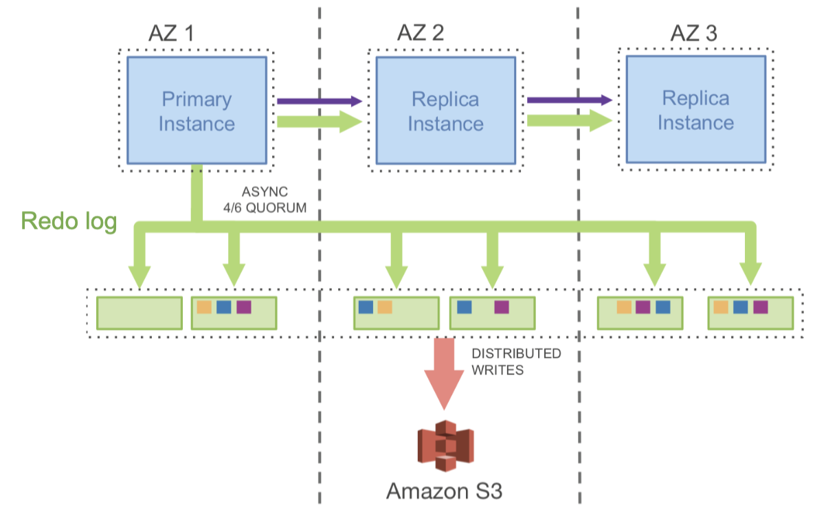
  • Logging uses async quorum: wait until 4 of 6 nodes reply (faster than waiting for all 6)
  • Each storage node takes the log and rebuilds theDB pages locally
  • Care taken to handle incomplete logs due to async quorums
  • Other features
    • Rapidly add or remove read replicas
    • Serverless Aurora (onlypay when actively running queries)
    • Efficient DB recovery, cloning and rollback (use a prefix of the log and older pages)

OLAP - BigQuery

• Goal - cloud OLAP
• Interface - SQL, JDBC, ODBC, etc
• Consistency - depends on storage chosen (object stores or richer table storage)
• Traditional data warehouses - no elasticity
• BigQuery and other elastic analytics systems
  • Separate compute and storage
  • Users pay separately for storage & queries
  • Get performance of 1000s of servers to run a query, but only pay for a few seconds of use
• Results
  • These elastic services generally provide better performance and cost for ad-hoc small queries than launching a cluster
  • For big organizations or long queries, paying per query can be challenging, so these services let you bound total # of nodes
• Interesting challenges
  • User-defined functions (UDFs) - need to isolate across tenants (e.g. in separate VMs)
  • Scheduling - How to quickly launch a query on many nodes and combine results? How to isolate users from each other?
  • Indexing - BigQuery tries to mostly do scans over column-oriented files

ACID over object stores - Delta Lake (Databricks)

• Motivation - Object stores are the largest, most cost effective storage systems, but their semantics make it hard to manage mutable datasets
• Goal - analytical table storage over object stores, built as a client library (no other services)
• Interface - relational tables with SQL queries
• Consistency - serializable ACID transactions
• Problems with naive “Just Objects”
  • No multi-object transactions
    • Hard to insert multiple objects at once(what if your load job crashes partway through?)
    • Hard to update multiple objects at once(e.g. delete a user or fix their records)
    • Hard to change data layout & partitioning
  • Poor performance
    • LIST is expensive (only 1000 results/request!)
    • Can’t do streaming inserts (too many small files)
    • Expensive to load metadata (e.g. column stats)
• Delta Lake's implementation
  • Can we implement a transaction log on top of the object store to retain its scale & reliability but provide stronger semantics?
  • Table = directory of data objects, with a set of log objects stored in _delta_log subdir
    • Log specifies which data objects are part of the table at a given version
  • One log object for each write transaction, in order: 000001.json, 000002.json, etc
  • Periodic checkpoints of the log in Parquet format contain object list + column statistics
  • Other features from this design
    • Caching data & log objects on workers is safe because they are immutable
    • Time travel - can query or restore an old version of the table while those objects are retained
    • Background optimization - compact small writes or change data ordering (e.g. Z-order) without affecting concurrent readers
    • Audit logging - who wrote to the table
• Other "bolt-on" (bolt-on causal consistency) systems
  • Apache Hudi (at Uber) and Iceberg (at Netflix) also offer table storage on S3
  • Google BigTable was built over GFS
  • Filesystems that use S3 as a block store (e.g. early Hadoop s3:/, Goofys, MooseFS)

Conclusion

• Elasticity with separate compute & storage
• Very large scale
• Multi-tenancy - security, performance isolation
• Updating without regressions

1.1.10. Streaming Systems

Motivation - Many datasets arrive in real time, and we want to compute queries on them continuously (efficiently update result)

All five letters - Kafka, Storm, Flink, Spark

Streaming query semantics

Streams

• Def - A stream is a sequence of tuples, each of which has a special processing_time attribute that indicates when it arrives at the system. New tuples in a stream have non-decreasing processing times.

  • event_time (in reality, may be out-of-order), processing_time

• Bounding event time skew

  • Some systems allow setting a max delay on late records to avoid keeping an unbounded amount of state for event time queries
  • Usually combined with “watermarks”: track event times currently being processed and set the threshold based on that

Stanford CQL (Continuous Query Language)

• “SQL on streams” semantics based on SQL over relations + stream ⟷relation operators

  

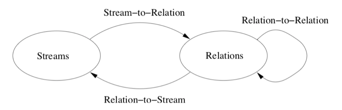
• Stream-to-Relation ops

  • Windowing - select a contiguous range of a stream in processing time (by time, tuples, partitions)
  • Many downstream operations could only be done on bounded windows!

• Relation-to-Relation ops - normal SQL

• Relation-to-Stream ops

  • Capture changes in a relation (each relation has a different version at each process time t)
  • ISTREAM(R),DSTREAM(R) contains a tuple (s, t) when tuple s was inserted/deleted in R at proc. time t.
  • RSTREAM(R) contain (s, t) for every tuple in R at proc. time time t

• Examples

  • SELECT ISTREAM(*) FROM visits [RANGE UNBOUNDED] WHERE page=“checkout.html”
  • Returns a stream of all visits to checkout
    1. convert visits stream to a relation via “[RANGE UNBOUNDED]” window
    2. Selection on this relation (σpage=checkout)
    3. convert the resulting relation to an ISTREAM (just output new items)

• Syntactic Sugar in CQL - automatically infer “range unbounded” and “istream” for queries on streams

• In CQL, every relation has a new version at each processing time

• In CQL, the system updates all tables or output streams at each processing time (whenever an event or query arrives)

Google Dataflow model

• More recent API, used at Google and open sourced (API only) as Apache Beam
• Somewhat simpler approach - streams only, but can still output either streams or relations
• Many operators and features specifically for event time & windowing
• Model - Each operator has several properties
  • Windowing - how to group input tuples (can be by processing time or event time)
  • Trigger - when the operator should output data downstream
  • Incremental processing mode - how to pass changing results downstream (e.g. retract an old result due to late data)

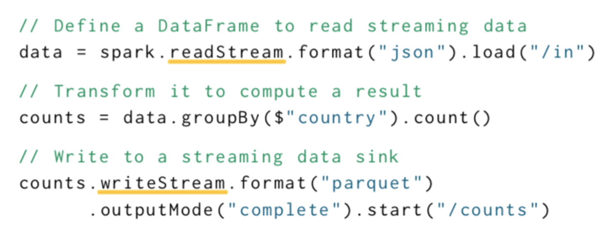
Spark Structured Streaming

• Even simpler model: specify an end-to-end SQL query, triggers, and output mode
• Spark will automatically incrementalize query
• Example Spark SQL batch query
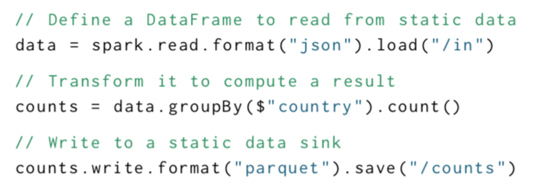
• Spark SQL streaming query
• Other streaming API features
  • Session windows - each window is a user session (e.g. 2 events count as part of the same session if they are <30 mins apart)
  • Custom stateful operators - let users write custom functions that maintain a “state” object for each key

Outputs to other systems

• Transaction approach - streaming system maintains some “last update time” field in the output transactionally with its writes
• At-least-once approach - for queries that only insert data (maybe by key), just run again from last proc. time known to have succeeded

Query planning & execution

How to run streaming queries?

1. Query planning - convert the streaming query to a set of physical operators - Usually done via rules
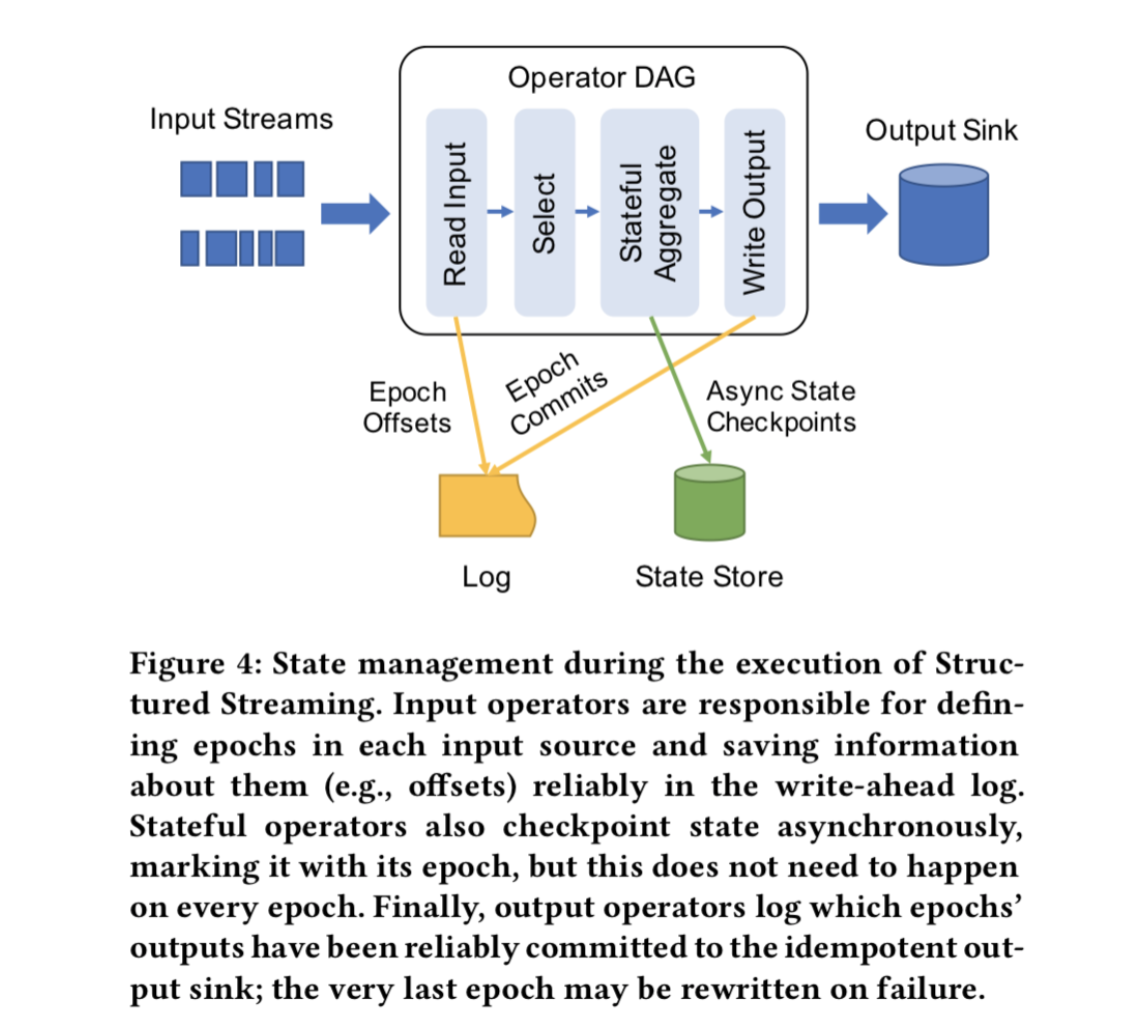
2. Execute physical operators - Many of these are “stateful”: must remember data (e.g.counts) across tuples
3. Maintain some state reliably for recovery - Can use a write-ahead log

Query planning - “incrementalize” a SQL query?

Fault tolerance

Need to maintain

• What data we outputted inexternal systems (usually, up to which processing time)
• What data we read from each source at each proc. time (can also ask sources to replay)
• State for operators, e.g. partial count & sum

What order should we log these items in?

• Typically must log what we read at each proc. time before we output for that proc. time
• Can log operator state asynchronously if we can replay our input streams

Example - structured streaming

Parallel processing

• Required for very large streams, e.g. app logs or sensor data
• Additional complexity from a few factors (with typical implementation)
  • How to recover quickly from faults & stragglers?
    • Split up the recovery work (like MapReduce)
  • How to log in parallel?
    • Master node can log input offsets for all readers on each “epoch”
    • state logged asynchronously
  • How to write parallel output atomically?(An issue for parallel jobs in general; see Delta)
    • Use transactions or only offer “at-least-once”

Summary

• Streaming apps require a different semantics
• They can be implemented using many of the techniques we saw before
  • Rule-based planner to transform SQL ASTs into incremental query plans
  • Standard relational optimizations & operators
  • Write-ahead logging & transactions

1.1.11. Review

Typical system challenges

• Reliability - in the face of hardware crashes, bugs, bad user input, etc
• Concurrency: access by multiple users
• Performance: throughput, latency, etc
• Access interface: from many, changing apps
• Security and data privacy

Two big ideas: declarative interfaces & transactions

Key concepts

• Arch
  • Traditional RDBMS:self-contained end to end system
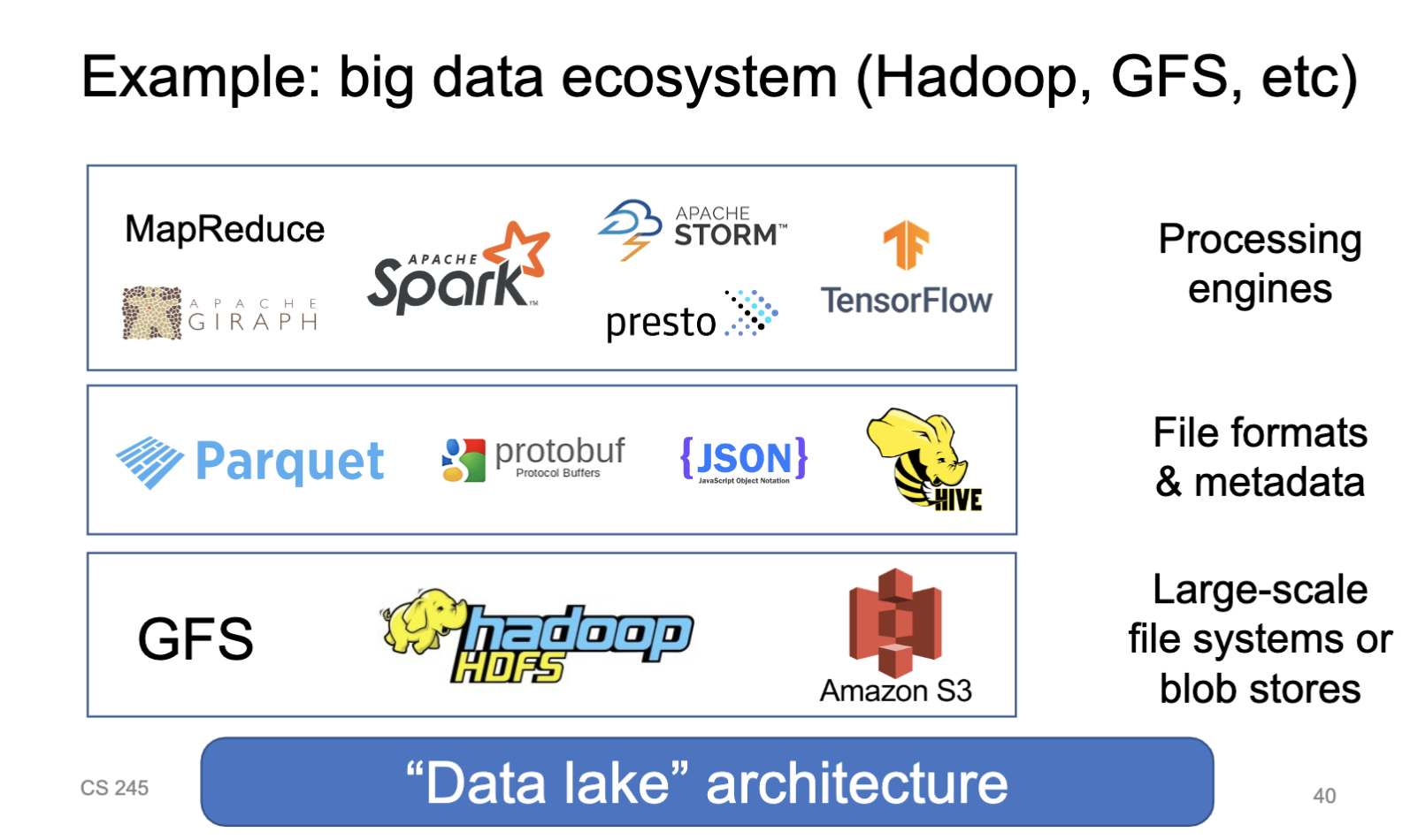
  • Data lake - separate storage from compute engines to let many engines use same data
• Hardware
  • Latency, throughput, capacity
  • Random vs sequential I/Os
  • Caching & 5-minute rule
• Storage
  • Field encoding
  • Record encoding - fixed/variable format, etc.
  • Table encoding - row/column oriented
  • Data ordering
  • Indexes - dense/sparse, B+-trees/hashing, multi-dimensional
• Query execution
  • Query representation - e.g. SQL
  • Logcial query plan - relational algebra
  • Optimized logical plan
  • Physical plan - code/operators to run
    • Many execution methods - per-record exec, vectorization, compilation
• Relational algebra
  • ∩, ⋃, –, ⨯, σ, P, ⨝, G
• Optimation
  • Rule-based: systematically replace some expressions with other expressions
  • Cost-based: propose several execution plans and pick best based on a cost model
  • Adaptive: update execution plan at runtime
  • Data statistics: can be computed or estimated cheaply to guide decisions
• Correctness
  • Consistency constraints: generic way to define correctness with Boolean predicates
  • Transaction: collection of actions that preserve consistency
  • Transaction API: commit, abort, etc
• Recovery
  • Failture models
  • Undo, redo, undo/redo logging
  • Recovery rules for various algorithms (including handling crashes during recovery)
  • Checkpointing and its effect on recovery
  • External actions → idempotence, 2PC
• Concurrency
  • Isolation levels, especially serializability
    • Testing for serializability: conflict serializability, precedence graphs
  • Locking:lock modes, hierarchical locks, and lock schedules (well formed, legal, 2PL)
  • Optimistic validation:rules and pros+cons
  • Recoverable, ACR & strict schedules
• Distributed
  • Partitioning and replication
  • Consensus: nodes eventually agree on one value despite up to F failures
  • 2-Phase commit: parties all agree to commit unless one aborts (no permanent failures)
  • Parallel queries: comm cost, load balance, faults
  • BASE and relaxing consistency
• Security & privacy
  • Threat models
  • Security goals: authentication, authorization, auditing, confidentiality, integrity etc.
  • Differential privacy: definitions, computing sensitivity & stability
• Putting all together
  • How can you integrate these different concepts into a coherent system design?
  • How to change system to meet various goals (performance, concurrency, security, etc)?